Sometimes, Noise Helps

I’ve been working on a fun problem lately that involves estimating a scalar parameter from a set of repeated observations. It turns out that in certain circumstances, the presence of noise in the system can actually make the estimate more accurate, which is a little counterintuitive and also kind of cool.

In my case, I have a number of observations (pixels), and I am trying to analyze a large number of them to estimate the parameter of interest. The image capture system I’m using quantizes the incident light into 8 bits per pixel — that is, to an integer between 0 and 255. However, I have reason to believe that the underlying analog sensor is fundamentally more accurate than the quantizer’s step size, and I would like to recover the most accurate possible value for the parameter.

The diagram below abstracts the problem:

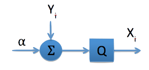
Here alpha is the parameter I want to estimate, the Y_i values are noise, Q represents the quantizer, and the X_i values are the observations available to my estimator. Can it be that my estimator will perform better in the presence of noise than in its absence?

Let’s assume that the quantizer is uniform and that analog values are rounded off to the nearest integer. The diagram below helps to visualize Q’s operation.

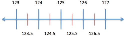
We’ll call the integer values, indicated by the blue vertical lines, the reconstruction levels. These are the outputs of the quantizer. We’ll call the values corresponding to the red lines the decision levels. The quantizer operates by determining between which two decision levels a value lies, and then outputting the reconstruction level between the same two decision levels. For example, if the value to be quantized is 126.4, the quantizer determines that the value lies between 125.5 and 126.5 and outputs 126. (Not to digress too far into quantization theory, but if the marginal distribution of the random process being quantized isn’t uniform, a uniform spacing of the decision levels is not optimal in a mean-square sense).

Now, how about my problem of estimating alpha? Let’s assume alpha is a constant 126.4. If there is no noise, then every X_i value will be identical and equal to 126. There is no reason to estimate alpha as anything other than 126. In the absence of noise, the quantizer limits my ability to estimate alpha. However, if noise is added to each observation, then nearby integers will also be output by the quantizer: 124, 125, 127, 128 etc. It’s reasonable to ask if the mean of the X_i observations will yield a better estimate.

To approach this analytically we need to make some assumptions about the noise. We’ll make life easy and assume the Y_i values are independent identically distributed zero mean normally distributed random variables. In this case, it is easy to write a script for computing the expected value of the quantizer’s output: E. For those interested in the computation, the accompanying python script provides the details. In practice, we would observe as many of the X_i values as we can, average them together, and use that average as our estimate. The average should converge to E as more and more observations are made.

The graph below, where alpha is set to 123.4, shows how noise helps. Clearly, as the standard deviation of the noise increases, the estimate becomes better. Fast. With a standard deviation as small as 0.5 the estimate is essentially perfect.

Fortunately for me, there is noise in my image capture system, and I have thousands and thousands of pixels over which to average, so my estimate can converge to E.